Wildlife Tracking Home

Automated Processing of Large Amounts of Thermal Video Data from Free-living Nocturnal Rodents

Christian Bankester (Department of Mathematics, LSU)
Sebastian Pauli (Department of Mathematics and Statistics, UNCG)
Matina Kalcounis-Rueppell (Department of Biology, UNCG)

October 2011

This page is based on a poster presented at the Conference of Research Experiences for Undergraduates Student Scholarship in October 2011.

Abstract

The study of animal behavior of nocturnal and elusive animals such as rodents is hindered by our lack of ability to see inspaniduals behaving naturally in their environment. New technologies such as thermal imaging allow us to remotely eavesdrop on the behaviors of nocturnal rodents. However, analyzing thermal video data is difficult because, although hundreds of hours of video data contain a wealth of information, the data cannot be processed efficiently by human observers. Using video data remotely collected from live oak riparian habitat in coastal California we applied the techniques of background subtraction, blog tracking and track analysis to examine behavior. At the study site, two species of Peromyscus (P. californicus and P. boylii) that differ in body size are the dominant resident species. We found that the behaviors and habitats are ripe with large amounts of animal behavioral detail. Our program provides an automated option to process large amounts of thermal video data collected from free living mice. The application of our program extends far beyond the confines of this research project. This program could have contributions in effectively any field where moving objects are filmed which require data extraction and analysis.

Introduction

Animal behavior is a major discipline in biology. The majority of studies have focused on those animals that are easiest to see and hear (ie, birds). However, the majority of mammals are nocturnal and elusive (ie, rodents), making it very difficult to examine their behavior. New technologies such as thermal imaging allow us to remotely eavesdrop on the behaviors of nocturnal rodents. However, analyzing thermal video data is difficult because, although hundreds of hours of video data contain a wealth of information, the data cannot be processed efficiently by human observers. Moreover, associated demographic information needs to be applied to the video data to make meaningful observations about patterns of behavior. In our field studies, we have collected more than 1600 hours of data from a live oak riparian habitat in coastal California where two species of Peromyscus (P. californicus and P. boylii) that differ in body size are the dominant residents. The object of this study was to process these videos to extract meaningful behavioral data.

Approach

The track data obtained with computer vision techniques animals is processed to identify tracks of the same inspanidual. Then we use size, speed, and movement patterns to assign individuals to particular species. We validated our output by comparing behavioral patterns with output from those same videos that were completely annotated by a human observer.

The Program

Figure 1: The main steps in processing the video.

The video is first analyzed using background subtraction and blob tracking. Frame-by-frame, each moving blob's position is recorded. The tracking data is processed and the speed of the blobs is computed using data about the focal area from a spreadsheet. After the Track-joining step the tracking data and the notes of a human observer are compiled on an HTML page. Background subtraction and blob tracking were written using the libraries OpenCV and cvBlob. The processing and output routines were written in Python.

Figure 2: The video shows the original video, the background subtraction, the blob tracking, the data obtained from the blob tracking, and a plot of the resulting track.

Tracking

The tracking of individuals in the videos is done in several steps

1. Background subtraction
2. Image clean up
3. Blob detection and labeling
4. Blob tracking

In the background subtraction step the mice (and other moving objects, such as rats) are isolated from the complex background, so that they can be seen as white moving blobs on a black background. We use the algorithm described in Liyuan Li, Weimin Huang, Irene Y.H. Gu, and Qi Tian Foreground Object Detection from Videos Containing Complex Background, ACM MM2003 implemented in OpenCV. Unfortunately this resulting video quite often still has minor disturbances we remove in the clean up step. In this step we also dilate the image, such that blobs that belong to the same individual are merged.

In the third step the blobs are recognized and their movements is tracked. The tracking data for each frame of the video the tracking function returns a list of all blobs together with their position and a bounding box for the blob. The blobs are identified with A linear-time component-labeling algorithm using contour tracing technique by Fu Chang, Chun-Jen Chen and Chi-Jen Lu (Computer Vision and Image Understanding, 2003) mplemented in the C++ library cvBlob by Cristóbal Carnero Liñán. 

See Measuring Behaviors of Peromyscus Mice from Remotely Recorded Thermal Video Using a Blob Tracking Algorithm for details.

Track Joining

When a list of blobs is generated from a video, it is a list of times with what blobs were present (and where) during that time. We reorganized this list into a collection of blobs and used a method termed track-joining to make the list more efficient and weed out errant tracks. The motivation for track-joining is that some of the tracks may actually belong to one blob, but were not correctly tracked by the blob-tracking piece of the program, for instance if an animal went under a branch, or in some other way disappeared from the view of the camera. To achieve this, we pitted each track against every other track and ranked their joining based on the four characteristics of positional distance between the tracks, temporal distance between the tracks, average speeds of the two tracks and the direction the blob was moving where one track left off and the direction of the other track. The ratings for each were between -5 to 5, and weighted appropriately based on what is more important for the two tracks to be joined.

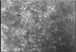
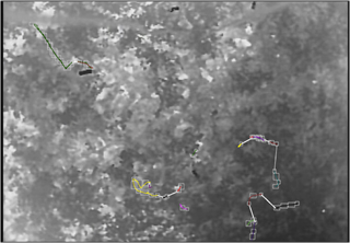
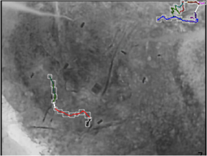
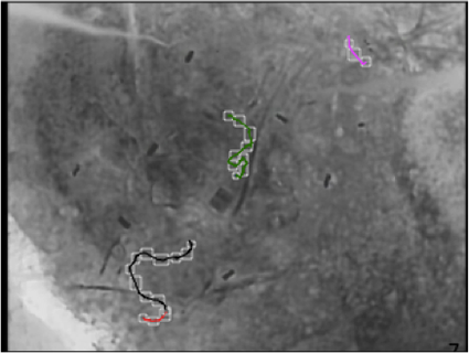
Figure 4 : The image on the left shows the output when track-joining is not used. The image on the right shows the data from the same video when track-joining is in place.

Visualization of tracks from long videos

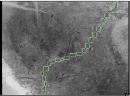
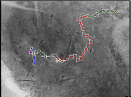
The videos we worked with for the development stage of this program were short (~1-5 minutes in length). This is not representative of the videos that the program was designed to work with, which are about three hours long. When a small video was processed, the small amount of activity allowed us to easily understand the graphical output. However, when a large video was processed, the increased activity in the video caused the graphical output to be very jumbled and hard to understand. To alleviate this problem, and make the image easier to understand, we broke up the output into several images. The points at which the output is broken up are determined by the amount of activity on the video at a given time, or by notes from human observation. This is illustrated in Figure 7.

Figure 5: The image above shows the graphical output before the output was broken up into several images, some which are displayed below.

459 to 699 seconds	699 to 824 seconds
824 to 923 seconds	1122 to 1143 seconds

Figure 6: .Each of the images is shown with the time interval in which it was taken from the video. This figure demonstrates the effectiveness of breaking up the output.

Output

To verify the data obtained from the tracking and track joining steps we output it together with the notes of a human observer on a HTML page. We visualize the computed imformation as a plot of tracks on top of a still from the video. This is realized as an HTML5 canvas. For a user selected time interval we show the tracks and the observers comments. The conversion of the data is done by a Python script.

Figure 7: A sample of the interactive output of the program. The image shows the focal image and the activity during the time interval shown in the top left corner. the time interval can be changed with the radio button on the top of the page. The comments generated from human analysis are included to help us verify the program's analysis of the video. Furthermore for each track segment the average speed in pixels per frame (30 fps) is given. By mousing over more detailed time and area information for the blobs on the tracks can be obtained. Because of the dilation of the blobs they are larger than the animals in the original video. Also fast moving animals such as birds and bats are followed by a smear on the video, therefore the bounding boxes of their blobs can appear much to large.

Discussion

Acknowledgements

The work on this project was supported by National Science Foundation (Grant IOB-0641530 and REU-0850465). We would like to thank the Office of Undergraduate Research of UNCG and in particular it's director Mary Crowe. We thank David Schuchart for the first version of the tracking program and Caitlin Bailey for annotating the videos. Thanks also go to all the students who worked in the field collecting data and the Hastings Natural History Reserve for all of their support of our field work.